
Welcome back, Excel adventurers, to the next thrilling stage of your journey with GifHow! You’ve successfully navigated the foundational techniques in Part 1, and we’re incredibly excited to see you back for more. The path to spreadsheet mastery is paved with continuous learning, and today, we’re unlocking another treasure trove of 10 indispensable tips – numbers 11 through 20 in our epic 40-tip quest!
Prepare to delve deeper, work smarter, and transform your data handling from a chore into a craft. These aren’t just tricks; they’re powerful strategies to make your spreadsheets more dynamic, your analysis more insightful, and your workflow smoother than ever. Let’s continue building your Excel expertise!
11. Enter the Same Data in Multiple Cells at Once
Manually typing the same content into multiple cells is tedious and inefficient—especially across large spreadsheets. Fortunately, Excel provides a shortcut.
Here’s how to do it efficiently:
- Select all the cells where you want to input the same data. You can click and drag, or hold
Ctrland click each cell individually. - Type your desired content directly into the final active cell (usually the last one selected).
- Instead of pressing
Enter, hitCtrl + Enter.
This command automatically populates every selected cell with the same data or formula—ideal for applying consistent headers, formulas, or placeholder text across a range.
12. Use Paste Special with Formulas for Smart Data Adjustments
When formatting numeric data, applying a percentage style can sometimes produce misleading results—turning a “1” into “100%,” for instance. If you actually want “1” to display as “1%,” you’ll need to divide all values by 100.
Here’s how to fix it using Paste Special:
- Type
100into an empty cell and copy it (Ctrl + C). - Select the data you want to adjust.
- Right-click and choose Paste Special.
- In the dialog box, select the Divide option, then click OK.
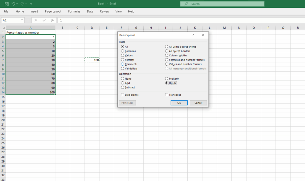
Excel will divide each selected cell by 100, correctly converting decimal numbers to percentage format. You can also use Paste Special for other quick math operations like multiplication, addition, or subtraction.
Here is the result
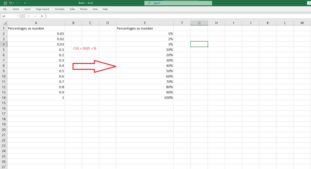
And you can convert to % form by pressing Ctrl + Shift + %
13. Save Charts as Templates for Reuse
Creating a well-designed Excel chart takes time. To avoid redoing formatting, styling, and customizations for future charts, save your current chart as a reusable template.
Steps to save and reuse a chart template:
- Right-click your finished chart.
- Select Save as Template.
- Save the file with a
.crtxextension in Excel’s default templates folder.
To apply your saved template:
- Select your new data.
- Go to the Insert tab → Recommended Charts → All Charts tab → Templates folder.
- Choose your saved template under My Templates and click OK.
Your new chart will retain fonts, colors, effects (like shadows or glows), and formatting—but note that text in titles or legends will only carry over if it’s tied to your data.
14. Add Graphics to Charts for Visual Impact
Make your data visually engaging by adding graphics or images to chart elements. Excel allows you to insert images into individual bars, pie slices, or columns for a more illustrative representation.
Here’s how to do it:
- Click the chart element (e.g., a pie slice or bar).
- Right-click and choose Format Data Point.
- In the Format Panel, choose Fill → Picture or texture fill.
- Upload a custom image or select from textures.
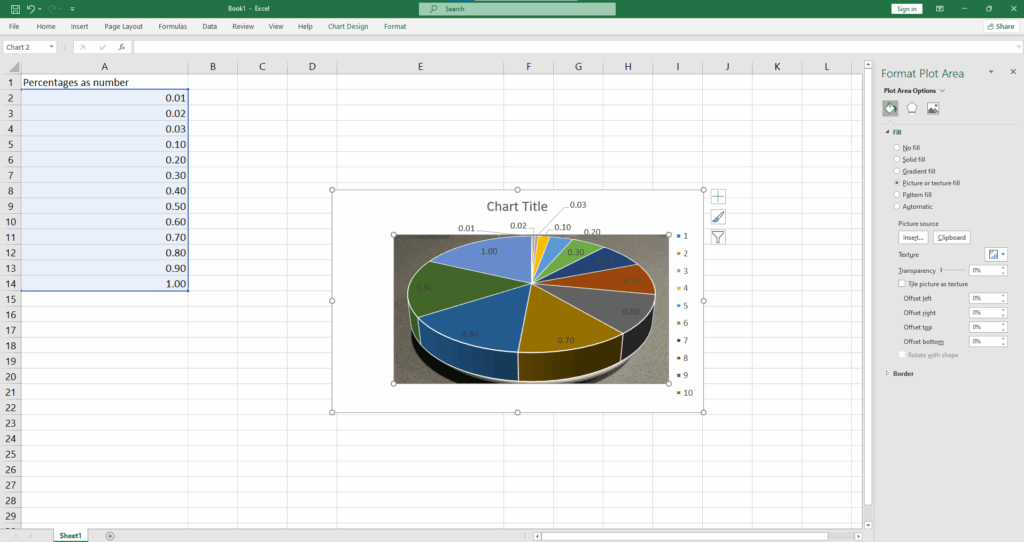
Use this to add icons, brand logos, or symbolic visuals (e.g., water drops for plumbing data). Just be cautious—too many graphics can clutter your chart and reduce readability.
You can access Make A graph in Excel by Gif How to watch video
15. Use 3D References Across Worksheets
When managing workbooks with identical layouts across multiple sheets (e.g., monthly budgets or annual reports), 3D references allow you to consolidate data without manual entry.
Example:
=SUM('Sheet1:Sheet12'!B3)This sums the values in cell B3 across all sheets from “Sheet1” to “Sheet12”.
You can also use other functions like AVERAGE, MAX, MIN, and COUNT with 3D references. It’s perfect for creating a summary or master sheet that updates dynamically with changes in the source sheets.
16. Hide Cell Values Without Deleting Them
Need to conceal data without affecting formulas? Instead of hiding an entire row or column, use custom formatting to make the contents invisible.
How to hide data within selected cells:
- Highlight the cells you want to hide.
- Right-click → Format Cells.
- In the Number tab, select Custom.
- In the Type field, enter:
;;;and click OK.
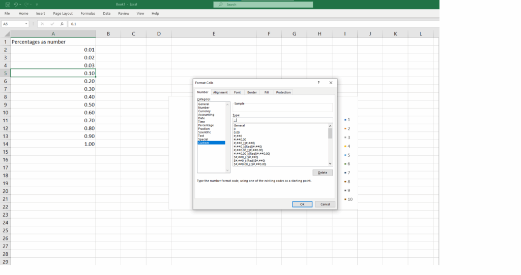
Now the values are invisible, but still exist—Excel can continue to use them in calculations and functions.
17. Hide Entire Worksheets (and Unhide Them Later)
When you want to keep a sheet in your workbook but don’t want it visible to others (or just to declutter), you can hide it without deleting any content.
To hide a worksheet:
- Right-click the sheet tab at the bottom and select Hide.
To unhide it:
- Go to the View tab → Unhide, then select the sheet you want to display.
For deeper control, Excel also allows you to hide the entire workbook window (via View → Hide). It looks like the file is closed, but it’s still active. You’ll need to Unhide it again before working with it.
18. Store Macros in Your Personal Workbook
Macros help automate repetitive tasks in Excel, but by default, they’re saved only within the file you created them in. If you want them available every time Excel opens—regardless of the file—you’ll need to use the Personal Macro Workbook.
How to do it:
- Enable the Developer tab (File → Options → Customize Ribbon → check “Developer”).
- Start recording a macro.
- In the Store macro in dropdown, choose Personal Macro Workbook.
Excel creates a hidden workbook named Personal.XLSB, which opens invisibly with Excel. Macros stored here are always available, making your automation tools universal across all workbooks.
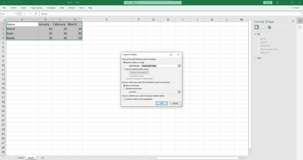
19. Master PivotTables to Summarize Data Efficiently
PivotTables are Excel’s most powerful tool for summarizing large datasets. They allow you to dynamically group, filter, and analyze data without complex formulas.
To create a PivotTable:
- Select your dataset (make sure it includes headers).
- Go to the Insert tab → click PivotTable.
- Choose whether to place the PivotTable in a new sheet or the current one.
- Drag and drop fields into Rows, Columns, Values, and Filters to configure your view.
And here is the result
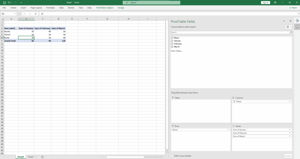
You can also try Recommended PivotTables to let Excel suggest layouts for you. Or use PivotCharts to add visual context.
20. Drill Down Into PivotTable Data
Ever wonder exactly where a value in your PivotTable came from? Excel lets you drill down and view the source data instantly.
To do this:
- Simply double-click on a PivotTable cell.
Excel will generate a new worksheet containing only the rows from your original data that contributed to that number. It’s a fast way to troubleshoot or audit your analysis and is especially helpful when dealing with grouped or filtered data.
Final Thoughts
Mastering these 10 Microsoft Excel tips will help you become more confident in handling your work, improving your performance and quality of work.
Happy spreadsheeting!