40 Sparkling Excel Hacks Every Busy Creator Should Know (Part 4)

Welcome back to Gif.How, You’ve been on an incredible journey with us, exploring the vast capabilities of Microsoft Excel. And guess what? We’re about to cross the finish line!

In Parts 1, 2, and 3, we laid some serious groundwork. Now, in this final installment, we’re completing your skillset with the last 10 game-changing techniques. These are the tips that will help you automate the most tedious tasks, navigate complex workbooks with ease, and even leverage the power of AI. Are you ready to become a true Excel master? Of course, you are! Let’s dive into the final chapter of your spreadsheet mastery!

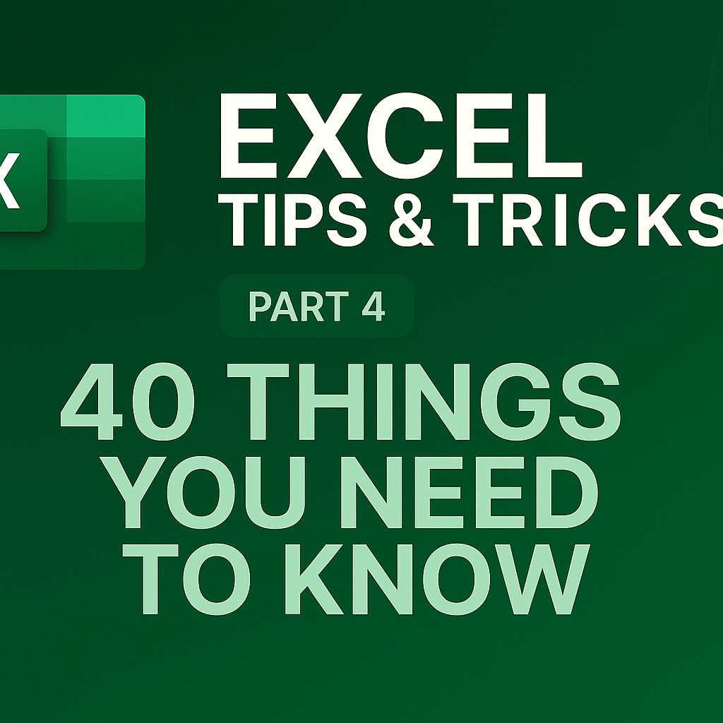
31. Quick Calculations Without Formulas: The Status Bar Secret

Got a bunch of numbers in a spreadsheet you want a quick calculation on without the hassle of creating a SUM formula in a new cell? Excel offers a much quicker way.

Harness the power of the status bar:

1. Click the first cell containing a number.
2. Hold down the Ctrl key and click the other cells you want to add.
3. Look down at the status bar at the very bottom of the Excel window. You’ll see the Sum of the selected cells calculated and displayed for you automatically.

Even better, right-click the status bar to open the Customize Status Bar menu. Here, you can add other quick calculations like Average, Count (to count how many cells you’ve selected), or Numerical Count (to count only the cells that contain numbers).

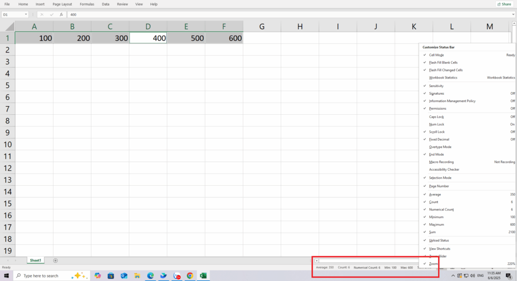
32. Freeze Panes: Keep Your Headers in Sight

Working with a massive dataset can be difficult, especially when you scroll up and down or left and right and lose track of what a column or row is about. There’s a simple trick for that: freeze the header row or column.

Here’s how to keep your headers locked in place:

1. Go to the View tab on the ribbon.
2. Click on Freeze Panes.
3. You’ll have several options:
   • Freeze Top Row: Locks the top row.
   • Freeze First Column: Locks the first column.
   • Freeze Panes: To freeze both rows and columns, click the cell that is immediately below your header row and to the right of your header column (e.g., cell B2 to freeze row 1 and column A). Then, select this option. All rows above and all columns to the left of your selected cell will be frozen.

When you want to remove the freeze, simply go back to the menu and select Unfreeze Panes.

See more How to Freeze Multiple Rows in Excel at Gif.How

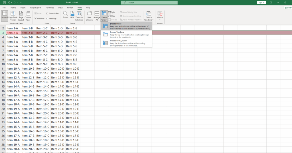
33. New Window: Get a Dual View of Your Sheet

Spreadsheets can become enormous. Sometimes you need to interact with different areas of the same sheet, such as copying and pasting info from the top to the bottom. The constant scrolling can make you dizzy. Instead, just open a second window with a view of the exact same spreadsheet.

See your sheet from two angles:

1. In the View tab, click New Window.
2. A new window containing your exact spreadsheet will open.
3. Click Arrange All (also in the View tab) to organize your windows neatly on the screen (e.g., side-by-side).

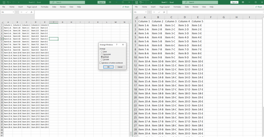
Now, when you type anything in one window, it will instantly appear in the other. This trick is especially handy if you use dual monitors.

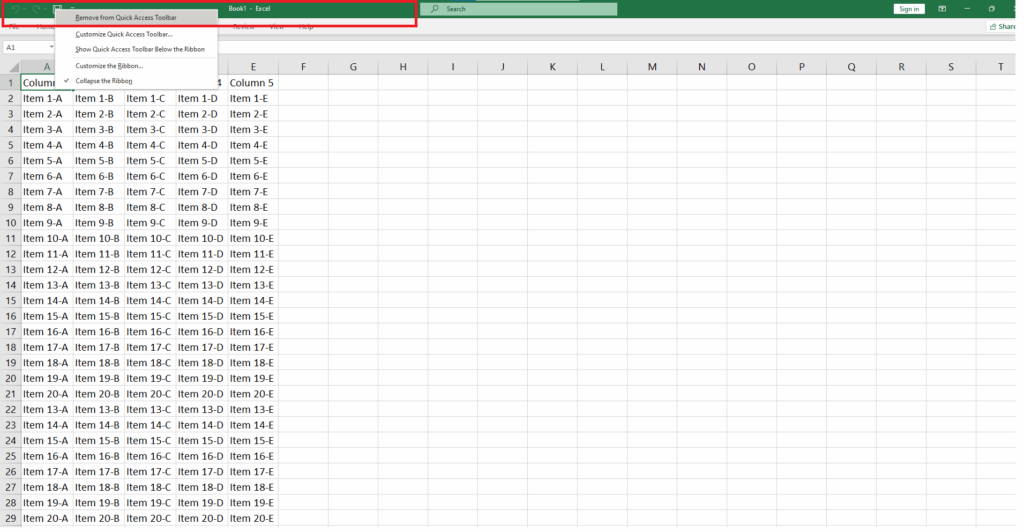
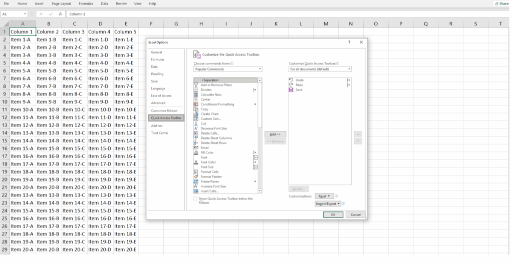
34. Customize the Quick Access Toolbar: Your Personal Command Center

The Quick Access Toolbar usually sits at the very top of the Excel window, with just a few buttons like Save, Undo, and Redo. But you can turn it into a powerhouse command center filled with your most-used shortcuts.

Build your custom toolbar:

1. Go to ToolBar> Right-Click>Customize Quick Access Toolbar.
2. On the left, you’ll see a list of commands. You can choose from “Popular Commands” or click the dropdown menu to select commands from any tab, or even All Commands to see the entire catalog.
3. Select a command you want and click Add >>.
4. That command will now appear on your toolbar. You can even add macros you’ve created for one-click access!

35. Format Multiple Tabs at Once: Synchronize Your Style

Let’s say you want to apply the same formatting to multiple worksheets—for example, you want the first row in every tab to be bold. Instead of doing it manually one by one, you can group them.

Here’s how:

1. Click the tab of the first sheet you want to format.
2. Hold down the Ctrl key and click the other tabs you want to select.
3. Now, any formatting you apply to the active sheet (e.g., changing a color, bolding text in cell A1) will be applied to the same cell in all the selected sheets.

36. Hyperlink Hero: Effortless Navigation Between Sheets

A workbook can contain dozens of sheets, and navigating between them can be a pain. Create hyperlinks to jump around instantly.

How to create a navigational link:

1. Select a cell where you want to place the link.
2. Right-click and select Link (or go to the Insert tab > Link).
3. In the pop-up dialog box, select Place in This Document.
4. You can then choose the sheet you want to link to and even specify a particular cell (like A1) on that sheet.
5. Type the text you want the link to display in the “Text to display” box.

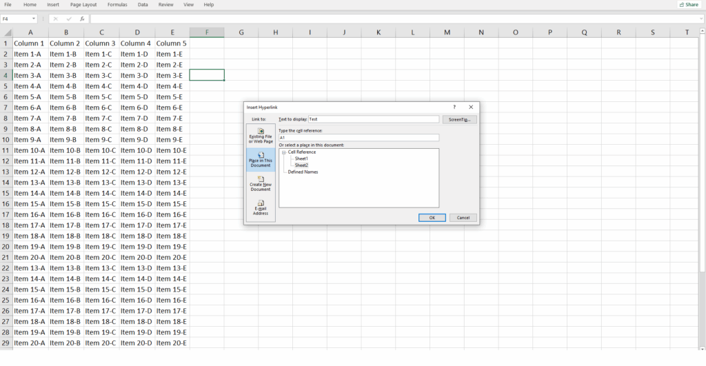
Now you can create a “Table of Contents” on your first sheet to quickly jump to any part of your workbook.

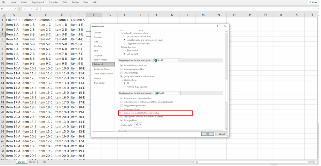
37. Declutter Your Data: Hide Unwanted Zeros

A spreadsheet full of numbers might have many cells with a value of zero. Sometimes, to make the data more readable, you want these zeros to simply disappear, leaving the cell blank.

How to hide the zeros:

1. Go to File > Options > Advanced.
2. Scroll down to the section Display options for this worksheet.
3. Uncheck the box that says Show a zero in cells that have zero value.
4. Click OK. All the zeros in that worksheet will vanish from view, making your data look much cleaner.

38. Master XLOOKUP: The Modern Way to Find Data

If you’ve been using Excel for a while, you’re likely familiar with VLOOKUP. In 2019, Microsoft introduced its powerful successor: XLOOKUP. Mastering this function is a true game-changer that can elevate your Excel skills to a professional level. (Pro-tip: HR departments and data analysts are actively looking for people with this skill!)

The major improvement is XLOOKUP‘s flexibility. It can look for data vertically and horizontally, search from right-to-left or left-to-right, and is less prone to errors when you insert or delete columns. It effectively replaces both VLOOKUP and HLOOKUP, and even the more complex INDEX/MATCH combination.

Here’s the basic concept of how it works:

The function asks Excel to find a specific item in one range (a column or a row) and then return a corresponding item from another range.

The basic structure is: =XLOOKUP(lookup_value, lookup_array, return_array)

• lookup_value: The item you are looking for (e.g., an employee’s name).
• lookup_array: The column or row where Excel should search for that item (e.g., the column of employee names).
• return_array: The column or row from which you want to pull the result (e.g., the column of salaries).

XLOOKUP also has powerful optional arguments for handling errors (what to do if the value isn’t found) and performing more advanced searches. While this video from Microsoft gives a quick overview, there are hundreds of excellent tutorials on YouTube that will help you master this essential function.

See more How to Use a VLOOKUP in Excel Easily at Gif.How

39. Leverage Your AI Assistant: Get Ahead with Copilot

Artificial intelligence is now integrated into Excel through Copilot. If you have a Microsoft 365 and Copilot Pro subscription, you can ask the AI to do incredible things.

To get started, ensure your file is saved on OneDrive or SharePoint with AutoSave turned on. Then, click the Copilot icon on the ribbon. You can ask it to:

• Analyze your data and suggest charts.
• Create complex formula columns.
• Highlight key trends and insights.

40. AI as Your Formula Guru: Ask and You Shall Receive

Even if you don’t have Copilot Pro, you can still use the power of AI to create Excel formulas. Any generative AI—like ChatGPT, Google’s Gemini, or the free versions of Copilot—can help you.

How to use AI for formulas:

1. Open your favorite AI chatbot.
2. Describe what you need clearly and specifically. For example: “Write me an Excel formula that sums the values in column B only when the corresponding value in column A is ‘Revenue’.”
3. The AI will give you the formula, often with an explanation of how it works.
4. Copy and paste the formula into the appropriate cell in your spreadsheet. Just remember to double-check it to make sure it works correctly.

And that’s a wrap! 40 sparkling Excel hacks are now in your toolkit. We at Gif.How are thrilled to have been on this learning adventure with you. Take the time to practice, because the real magic happens when you apply this knowledge to your own projects.

Which of these tips has already changed your workflow? Share your thoughts and discoveries in the comments below!

You may also be interested in

• 40 Sparkling Excel Hacks Every Busy Creator Should Know (Part 3)
• 40 Sparkling Excel Hacks Every Busy Creator Should Know (Part 2)
• 40 Sparkling Excel Hacks Every Busy Creator Should Know (Part 1)
• Excel – gif.how