Ever found yourself scrolling through a massive Excel sheet, only to completely lose track of your column headers? It’s like reading a book without a title – confusing and inefficient! Whether you’re tracking sales, managing inventory, or just organizing your finances, losing sight of those crucial top rows can turn a simple task into a frustrating hunt.
But what if you could keep your headers visible, no matter how far down you scroll? Good news, you absolutely can! Excel has a super handy feature that lets you “freeze” specific rows (or even columns) so they stay put while the rest of your data moves freely. This little trick is a game-changer for anyone who spends time in spreadsheets.
Ready to make your Excel experience smoother and much less frustrating? Let’s dive into how you can easily keep those important top rows right where you can see them.
Why Freezing Rows Will Change Your Excel Life
Imagine you have a long list of customer orders. Each column has a header: “Order ID,” “Customer Name,” “Product,” “Quantity,” “Price,” etc. As you scroll down to look at order #500, those headers disappear. You then have to scroll back up just to remember if column D is “Quantity” or “Price.” Annoying, right?
Freezing rows solves this instantly. Your “Order ID,” “Customer Name,” and other headers will always be at the top of your screen, no matter how far you go down your list. This means less scrolling back and forth, fewer mistakes, and a much clearer view of your data. It’s all about making your work flow better and keeping you focused on what matters.
How to Freeze a Row in Excel: The Quick Guide
The process is surprisingly simple, and once you know it, you’ll wonder how you ever lived without it. Here’s a quick breakdown:
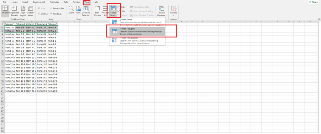
- Select the row below the one you want to freeze. For example, if you want your first row (Row 1) to stay visible, click on Row 2. Excel will freeze everything above your selection.
- Go to the “View” tab in the Excel ribbon.
- Look for the “Freeze Panes” button in the “Window” group.
- Click on “Freeze Panes.”
And just like that, your top row (or rows, depending on your selection) will be locked in place! Now try scrolling down – your headers should stay perfectly still.
See It in Action!
Sometimes, seeing is believing. We’ve put together a super short, easy-to-follow video that walks you through freezing rows in Excel step-by-step. It’s the quickest way to get this skill down pat and start making your spreadsheets work smarter for you.
Watch the short video guide on how to freeze rows in Excel here! (You’ll link this to your specific GIF.how video page)
Beyond the Basics: Unfreeze and Freeze First Column
What if you change your mind, or need to unfreeze the rows?
- Just go back to the “View” tab, click “Freeze Panes”, and then select “Unfreeze Panes.” Easy peasy!
And if you ever need to keep your first column visible while scrolling horizontally, Excel can do that too! Just choose “Freeze First Column” from the “Freeze Panes” dropdown menu.
Making your data easier to manage is what it’s all about. Freezing rows is a small trick that makes a huge difference in your daily Excel tasks. Give it a try, and enjoy a much smoother spreadsheet experience!
You just mastered a fantastic Excel shortcut that’ll save you tons of scrolling! Keeping your important headers visible is a game-changer for clarity and efficiency. Ready to unlock even more spreadsheet power? We also have super simple guides on how to freeze columns (perfect for wide datasets!) and even how to freeze both rows and columns at the same time. Check them out and make your Excel experience truly seamless! See more at Gif.How